What to do when backpressure increases?

An increase in back-pressure usually suggests either a guard or analytical column problem. To find exactly where the problem lies we suggest you remove the guard column (if you are using one) and replace the old cartridge with a new one.

If the original pressure is restored, you solved the problem.

If the pressure remains high, disconnect the analytical column from the system, backflush it (do NOT connect the column to the detector while doing so) and run a few column volumes of your mobile phase through the column.

If the problem still persists you may have some strongly retained contaminants in your column coming from your previous injections.
Run the appropriate restoration procedures, as suggested by the column manufacturer, and retest the column.

If the initial pressure is not restored you may have to change the inlet frit or replace the column.

Always run your system (2 to 5 ml/min) without the guard column and the analytical column to verify that your pressure isn’t coming from another source, like a blocked in-line column prefilter, blocked/kinked tubing, particulates blocking your injector etc.
Always work your way from the detector back to the pump to isolate the problem.

 

Tailing factor ,Efficiency calculation , Resolution and Symetry

 

Column efficiency calculation

Column efficiency, indicated as the number of theoretical plates per column, is calculated as N = 5.54 (t_R / w_0.5)² where t_R is the retention time of the analyte of interest and w_0.5 the width of the peak at half height.

This half-height method enables the determination of the number of theoretical plates per column (N) even if the peak is not fully separated from a neighbouring peak (poor resolution), as long as the valley between the peaks is lower than the half-height of the peak. Half-height measurements commonly is the method of choice for automatic determination by data systems.

The larger the number of theoretical plates per column, the sharper the peak! Should you need to calculate the number of theoretical plates per meter, you must use the following equation:

Number of theoretical plates per column x 100/length of HPLC column (cm)= Number of theoretical Plates per m

 

Peak Asymmetry Factor

Peak Asymmetry Factor, often presented as A_s is calculated with the following equation A_s = b/a where b is the distance from the peak midpoint (perpendicular from the peak highest point) to the trailing edge of the peak measured at 10% of peak height and a is the distance from the leading edge of the peak to the peak midpoint (perpendicular from the peak highest point) measured at 10% of peak height. If As > 1 : tailing, et si As < 1 : fronting

 

Tailing Factor

Tailing Factor (T_f) is the USP coefficient of the peak symmetry. It is calculated using the following equation: T_f = (a+b)/2a where a is the distance from the leading edge of the peak to the peak midpoint (perpendicular from the peak highest point) measured at 5% of peak height and b is the distance from the peak midpoint (perpendicular from the peak highest point) to the trailing edge of the peak measured at 5% of peak height.

 

Resolution

Resolution (R_s) is a measure of the separation quality. In order to determine the resolution between 2 peaks we need to measure the retention times of the 2 peaks of interest (t_r2 and t_r1) and the width of the 2 peaks at baseline (w₁ and w₂) between tangents drawn to the sides of the peaks. It is normally calculated as:

R_ss = (t_r2 – t_r1) / ((0.5 * (w₁ + w₂)

 

Since nearly every peak shows some degree of tailing, so to allow for a small amount of tailing and still retain a bit of flat baseline between the peaks, R_s ≥ 2.0 generally is desired for proper resolution between 2 peaks of interest.

This equation is extremely convenient and gives good results for peak resolution calculations, but it is only useful when the peaks are resolved at baseline level. However, we are often confronted to situation where peaks are marginally separated. Peaks overlap at the bottom, and measurement of the peak width at baseline is virtually impossible.

In these cases, just like we measured the efficiency at mid peak height, the same approach can be used for the calculation of the resolution with the following equation:

R_s = (t_R2 – t_R1) / ((1.7 * 0.5 (w_0.5,1 + w_0.5,2))

where w_0.5,1 and w_0.5,2 are the peak widths measured at half the peak height. Note that the factor of 1.7 is added to the denominator to adjust for the difference in width at the half-height. The half-height technique is the way many data systems measure resolution, because it is simpler to measure than the baseline width.

The number of theoretical plates per column (performance)/symmetry factor/Tailing Factor/Resolution can and will change depending on the type of analysis and analytical conditions used.

Column Efficiency or Theoretical plate

Column Efficiency or Theoretical plate

At the beginning of a chromatographic separation the solute occupies a narrow band of finite width. As the solute passes through the column, the width of its band continually increases in a process called band broadening. Column efficiency pro- vides a quantitative measure of the extent of band broadening.

In their original theoretical model of chromatography, Martin and Synge2 treated the chromatographic column as though it consists of discrete sections at which partitioning of the solute between the stationary and mobile phases occurs. They called each section a theoretical plate and defined column efficiency in terms of the number of theoretical plates, N, or the height of a theoretical plate, H; where

              12.12

A column’s efficiency improves with an increase in the number of theoretical plates or a decrease in the height of a theoretical plate.

Assuming a Gaussian profile, the extent of band broadening is measured by the variance or standard deviation of a chromatographic peak. The height of a theoreti- cal plate is defined as the variance per unit length of the column

                                              12.13

where the variance, σ2, has units of distance squared. Because retention time and peak width are usually measured in seconds or minutes, it is more convenient to ex- press the standard deviation in units of time, τ, by dividing  by the mobile phase’s average linear velocity.

                                 12.14

When a chromatographic peak has a Gaussian shape, its width at the baseline, w, is four times its standard deviation, τ.

w = 4τ            …………………12.15

Combining equations 12.13 through 12.15 gives the height of a theoretical plate in terms of the easily measured chromatographic parameters tr and w.

                                     12.16

The number of theoretical plates in a chromatographic column is obtained by com- bining equations 12.12 and 12.16.

                                12.17

Alternatively, the number of theoretical plates can be approximated as

where w1/2 is the width of the chromatographic peak at half its height.

It is important to remember that a theoretical plate is an artificial construct and that no such plates exist in a chromatographic column. In fact, the number of theo- retical plates depends on both the properties of the column and the solute. As a re- sult, the number of theoretical plates for a column is not fixed and may vary from solute to solute. 

MOBILE PHASE DISCRIPTION AND PROPERTIES

MOBILE PHASE DISCRIPTION AND PROPERTIES

 Mobile phase has been rightly termed as the lifeline of the HPLC system. It plays the important role of transport of the sample through the separation column and subsequently to the detector for identification of the separated components.

Mobile phase is seldom a single solvent. It consists of combination of water with organic solvents, aqueous buffers with polar solvents or mixtures of organic solvents in desired proportions. The two operational modes commonly used are:

Isocratic mode – in the Isocratic mode the composition of the mobile phase remains constant throughout the analytical run ,i.e, the proportion of solvents in the mixture is pre-decided and remains unchanged during analysis

Gradient Elution – the composition is varied by the software through the analytical run in a predetermined mode and at the end of the run the proportion of solvents is different from the initial proportion.

The objective of using different solvent mixtures is to achieve the desired polarity of mobile phase for complete miscibility of the sample and control interaction of sample components with the stationary phase to achieve the desired degree of resolution of separated component peaks in the shortest possible time.

In order to meet the required objectives the mobile phase should have the following essential features:

• The sample should be fully soluble in the mobile phase. Any insolubility will result in flow restrictions. Always check sample solubility in mobile phase before injection into the system.
• Mobile phase components should be non-hazardous and non-toxic. They should not pose any health hazard to the operator.
• Mobile phase shouId be inert towards sample constituents and the stationary phase. Any reactions can lead to formation of insoluble suspensions which can result in column blockages.
• The mobile phase should not give its own response on passing through the detector. In other words the detector signals should reflect only the response of the sample constituents. This, however, is not applicable in bulk property detectors such as refractive index detector which respond to overall changes in refractive index of the mobile phase containing the eluting compound.
• The mobile phase should be affordable and the proportion of solvents used should make the analysis economically viable.

It is important to mix the solvents of specified purity and from same source to get consistency of results and also to adopt the same off-line mixing technique to avoid errors due to heat of mixing errors. In case buffers are to be used always adjust the pH of the aqueous phase prior to making up the final volume with the organic phase.

HPLC technique holds great promise for applications in diverse fields. Control of operational conditions including consistency of mobile phase will ensure repeatability of results.

The Role of pH IN MOBILE PHASE -

The pH of the mobile phase (eluent) is adjusted to improve component separation and to extend the column life. This pH adjustment should involve not simply dripping in an acid or alkali but using buffer solutions, as much as possible. Good separation reproducibility (stability) may not be achieved if buffer solutions are not used.

A buffer solution is prepared as a combination of weak acids and their salts (sodium salts, etc.) or of weak alkalis and their salts. Common preparation methods include: 1) dripping an acid (or alkali) into an aqueous solution of a salt while measuring the pH with a pH meter and 2) making an aqueous solution of acid with the same concentration as the salt and mixing while measuring the pH with a pH meter. However, if the buffer solution is used as an HPLC mobile phase, even small errors in pH can lead to problems with separation reproducibility. Therefore, it is important to diligently inspect and calibrate any pH meter that is used. This page introduces a method that does not rely on a pH meter. The method involves weighing theoretically calculated fixed quantities of a salt and acid (or alkali) as shown in the table below. Consider the important points below.

Denoting Buffer Solutions

A buffer solution denoted, "100 mM phosphoric acid (sodium) buffer solution pH = 2.1," for example, contains phosphoric acid as the acid, sodium as the counterion, 100 mM total concentration of the phosphoric acid group, and a guaranteed buffer solution pH of 2.1.

Maximum Buffer Action Close to the Acid (or Alkali) pKa

When an acetic acid (sodium) buffer solution is prepared from 1:1 acetic acid and sodium acetate, for example, the buffer solution pH is approximately 4.7 (near the acetic acid pKa), and this is where the maximum buffer action can be obtained.

Buffer Capacity Increases as Concentration Increases

The buffer capacity of an acetic acid (sodium) buffer solution is larger at 100 mM concentration than at 10 mM, for example. However, precipitation occurs more readily at higher concentrations.

Beware of Salt Solubility and Precipitation

The salt solubility depends on the type of salt, such as potassium salt or sodium salt. Salts precipitate out more readily when an organic solvent is mixed in.

In addition, avoid using buffer solutions based on organic acids (carboxylic acid) as much as possible for highly sensitive analysis at short UV wavelengths. Consider the various analytical conditions and use an appropriate buffer solution, such as an organic acid with a hydroxyl group at the α position  to restrict the effects of metal impurity ions

Differences in Preparation Method May Result in Different Chromatograms -

A water-based solvent, organic solvent, or a mixture of the two is mainly used as the mobile phase for HPLC. A buffer solution is often used as the aqueous solvent. describes the actual preparation methods for typical buffer solutions used with HPLC. However, it seems that many people have a vague understanding of buffer solutions.

If the preparation method is not the same as the method described in the material for the analysis method, differences can occur in the mobile phase that affect the chromatograms and analysis results. Apart from the buffer solution, many other unforeseen factors affect the mobile phase preparation, such as the method of mixing the solvent.

Here, we use actual examples to consider the effects of the mobile phase preparation method on the analysis results.

 Preparing Buffer Solutions

In practice, how do we go about preparing a buffer solution that is denoted as "20 mM phosphoric acid buffer solution (pH=2.5)"? Let's examine a few possible issues.
First, we know that it is a phosphoric acid buffer solution, but what is the counterion? If sodium ions are unambiguously the counterion, does "20 mM" refer to the phosphoric acid concentration or the sodium phosphate concentration?

For a 20 mM phosphoric acid (sodium) buffer solution, "20 mM" could be considered to be the phosphoric acid concentration. On the other hand, considering "20 mM" to be the sodium concentration, the buffer solution could be a buffer solution prepared by adjusting the pH using a 20 mM aqueous solution of sodium dihydrogen phosphate. (However, a 20 mM aqueous solution of sodium dihydrogen phosphate has a pH just under 5, so that pH adjustment with some type of acid is required to achieve pH 2.5.)
However, an ion-pair effect due to the acid used for pH adjustment could affect the analysis results. This is potentially dangerous, as it leads to several possible interpretations of a denoted buffer solution.

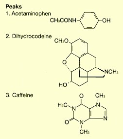
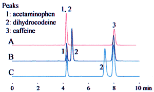
The example above leads to three potential interpretations. Fig. 1 shows how this affects the analysis results.
These differences can significantly affect the retention time, as shown for dihydrocodeine in the example, and can lead to problems with the robustness of the analysis method. Clearly identifying the buffer solution when specifying the preparation method can prevent problems due to differences in interpretation.

1. Acetaminophen 2. Dihydrocodeine 3. Caffeine